What are we doing here ?

Yeah, so recently I’ve been reading “The Man Who Solved The Market” by Gregory Zuckerman. Fun book about Jim Simons and his famously cracked Renaissance Technologies hedge fund. Unfortunately, it didn’t make me better at trading lol

BUT it motivated me to learn more about some of the maths they used. Notably, Markov chains are mentioned a few times, first in the context of the IDA, the (top-secret) Institute for Defense Analyses, where Simons worked before starting his fund and was free to pursue his own research while trying to crack the Russian codes. He published a paper about predicting stock prices using Markov chains.

Here is what Zuckerman says about it:

Simons and the code-breakers proposed a similar approach to predicting stock prices, relying on a sophisticated mathematical tool called a hidden Markov model. Just as a gambler might guess an opponent’s mood based on his or her decisions, an investor might deduce a market’s state from its price movements. Simons’s paper was crude, even for the late 1960s. He and his colleagues made some naive assumptions, such as that trades could be made “under ideal conditions,” which included no trading costs, even though the model required heavy, daily trading. Still, the paper can be seen as something of a trailblazer.

Also, one of his early associate, Lenny Baum, was the co-author of the Baum-Welch algorithm, a method for training hidden Markov models.

OK. That’s 2 instances. That’s more than enough justification to write a refresher on Markov chains and hidden Markov chains and try to implement some of the concepts in Python.

Markov Chains ?

It’s just a sequence of random variables where the probability of each variable depends only on the state attained by the previous variable (this is called the Markov property). That’s a big assumption. Formally, if we note the states of the system as $X_{0}, X_{1}, X_{2}, \ldots$, the Markov property states that for all $n \geq 0$ we have: $P(X_{n+1} | X_{n}, X_{n-1}, \ldots, X_{0}) = P(X_{n+1}| X_{n})$

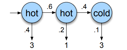
A Markov chain is usually represented by a graph :

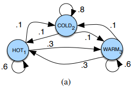
mchain — Each node is a possible state and each edge represents the transition probability.

And is entirely described by 3 components: an initial probability distribution $\pi$ , a transition probability matrix $$A$$ where each $a_{ij}$ represents the probability of moving from state $$i$$ to state $$j$$ and a list $$Q$$ of possible states $q_1 \ldots q_n$ .

If we circle back to our example, the list of our possible states is $Q = \{HOT, COLD, WARM\}$, the initial probability distribution could be $\pi = [0.1, 0.7, 0.2]$ and, by reading the graph, the transition matrix $A$ would be then:

$A = \begin{pmatrix} P(\text{HOT} \rightarrow \text{HOT}) & P(\text{HOT} \rightarrow \text{COLD}) & P(\text{HOT} \rightarrow \text{WARM}) \\ P(\text{COLD} \rightarrow \text{HOT}) & P(\text{COLD} \rightarrow \text{COLD}) & P(\text{COLD} \rightarrow \text{WARM}) \\ P(\text{WARM} \rightarrow \text{HOT}) & P(\text{WARM} \rightarrow \text{COLD}) & P(\text{WARM} \rightarrow \text{WARM}) \end{pmatrix}$ $A = \begin{pmatrix} 0.6 & 0.1 & 0.3 \\ 0.1 & 0.8 & 0.1 \\ 0.3 & 0.1 & 0.6 \end{pmatrix}$

This matrix represents the probabilities of moving from one state to another. The rows correspond to the current state (must sum to 1!), and the columns correspond to the next state.

Once we have that, we can perform some basic computations. For instance, if we want to find out the probability of the sequence $HOT \rightarrow HOT \rightarrow HOT \rightarrow HOT$, given our initial probability distribution $\pi = [0.1, 0.7, 0.2]$, that would be $0.1 \times 0.6^{3} \approxeq 2\%$. (Initial chance to be $HOT$ is $0.1$ then once we’re in the $HOT$ state we have $60\%$ chance of staying there…)

Hidden Markov Chains

A Hidden Markov Chain is like a Markov Chain, but with a twist: the states are hidden. You can’t directly observe the state the system is in; instead, you observe something that gives you a clue about the state.
Imagine now that instead of directly knowing the weather, you only get to know how many icecream someone ate. The weather (HOT, COLD) is still following a Markov chain, but you can only guess what the weather is based on the amount of icecream consumed (don’t ask why you can’t directly have access to the weather, just pretend).

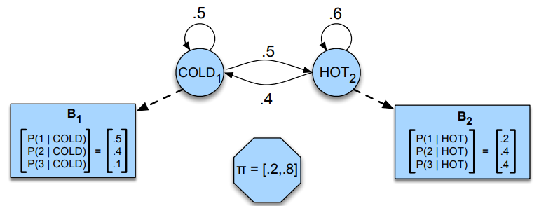
hmchain — The hidden states are represented by the circles and the possible observations with their associated probabilities by the squares.

A hidden Markov chain is entirely described by 4 components : an initial probability distribution $\pi$ , a transition probability matrix $$A$$ where each $a_{ij}$ represents the probability of moving from state $$i$$ to state $$j$$ , a list $$Q$$ of possible states $q_1 \ldots q_n$ and $$B$$ , the emission probability matrix where each $b_{ij}$ represents the probability of observing $O_{j}$ given that the system is in state $q_{i}$ .

The 3 fundamental problems

When dealing with Hidden Markov Models, we usually want to solve 3 things:

Likelihood: Given a model $\lambda = (A, B, \pi)$ and an observation sequence $O = O_{1}, O_{2}, \ldots, O_{T}$, how do we compute the probability $P(O \vert \lambda)$ that the model generates the observation sequence ?
Decoding: Given a model $\lambda = (A, B, \pi)$ and an observation sequence $O = O_{1}, O_{2}, \ldots, O_{T}$, how do we choose a sequence of states $Q = q_{1}, q_{2}, \ldots, q_{T}$ that best explains the observation sequence ?
Learning: Given an observation sequence $O = O_{1}, O_{2}, \ldots, O_{T}$, how do we adjust the model $\lambda = (A, B, \pi)$ to maximize the probability $P(O \vert \lambda)$ that the model generates the observation sequence ?

Let’s tackle these problems one by one.

Likelihood

Quite easy to understand, we just want to know how likely it is that the model generates a given observation sequence.
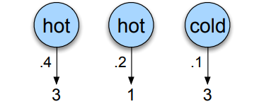
So for instance, if we continue our example and we want to know how likely it is that the model generates the sequence $3, 1, 3$ given the hidden states hot hot cold.
The computation would simply be $P(3, 1, 3 \vert \text{hot hot cold}) = P(3 \vert \text{hot}) \times P(1 \vert \text{hot}) \times P(3 \vert \text{cold})$ (thanks to Markov property), if we read the emission probabilities on our graph, we have $P(3 \vert \text{hot}) = 0.4$, $P(1 \vert \text{hot}) = 0.2$ and $P(3 \vert \text{cold}) = 0.1$, so the likelihood would be $0.4 \times 0.2 \times 0.1 = 0.008$.

The issue is that we don’t actually know the hidden states, so we also need to compute the probability that the hidden states were indeed hot hot cold which is given by : $P(\text{hot hot cold}) = P(\text{start} \rightarrow \text{hot}) \times P(\text{hot} \rightarrow \text{hot}) \times P(\text{hot} \rightarrow \text{cold})$ $P(\text{hot hot cold}) = P(\text{hot} \vert \text{start})\times P(\text{hot} \vert \text{hot}) \times P(\text{cold} \vert \text{hot})$ $P(\text{hot hot cold}) = 0.8 \times 0.6 \times 0.4 = 0.192$

If we piece everything together, we get can compute the joint probability of the observation sequence and the hidden states: $P(3, 1, 3, \text{hot hot cold}) = P(3, 1, 3 \vert \text{hot hot cold}) \times P(\text{hot hot cold}) = 0.008 \times 0.192 = 0.001536$

In general, for an observation sequence $O$ and a list of hidden states $Q$, the joint probability is given by: $P(O, Q) = P(O \vert Q) \times P(Q) = \prod_{t=1}^{T} P(O_{t} \vert Q_{t}) \times \prod_{t=1}^{T} P(Q_{t} \vert Q_{t-1})$

That’s cool, but that’s only for one possible sequence of hidden states. We need to compute this for all possible sequences and sum them up to get the actual likelihood of the observation sequence: $P(O) = \sum_{Q} P(O, Q) = \sum{Q} P(O \vert Q) \times P(Q)$

For us : $P(313) = P(313, \text{cold, cold, cold}) + \dots + P(313, \text{hot, hot, cold}) + \dots + P(313, \text{hot, hot, hot})$

Let’s do it in Python:

pi = np.array([0.2, 0.8])  # Initial state probability distribution

# 2 x 2 matrix because we have 2 states (1st state Cold, 2nd Hot)
A = np.array([[0.5, 0.5], 
              [0.4, 0.6]])  # Transition probabilities

O = [3, 1, 3]  # Observation sequence

# 2 x 3 matrix because we have 2 states and 3 possible observations encoded as 1, 2, 3 (number of icecreams)
B = np.array([[0.5, 0.4, 0.1], 
              [0.2, 0.4, 0.4]])  # Emission probabilities

import itertools
def naive_approach(pi, O, A, B):
    """
    pi: Initial state proability distribution (N)
    O: Observation sequence (length T)
    A: Transition probability matrix (N x N)
    B: Emission probability matrix (N x T)
    
    Enumerate all possible state sequences and compute the total probability 
    by summing the probabilities of each sequence
    """
    N = len(A)       # Number of states
    T = len(O)       # Length of observation sequence
    total_prob = 0
    # Enumerate all possible state sequences
    for state_seq in itertools.product(range(N), repeat=T):
        seq_prob = pi[state_seq[0]]  # Initial state probability
        # Probability of state transitions given by our transition matrix A
        for t in range(1, len(O)):
            seq_prob *= A[state_seq[t-1], state_seq[t]]
        # Probability of emissions given by our emission matrix B
        for t in range(T):
            seq_prob *= B[state_seq[t], O[t]-1]
        total_prob += seq_prob
    return total_prob

# naive_approach(A, B, pi, O)
# >> 0.0285

For long sequences, this approach is not feasible but smart people came up with the Forward Algorithm

Forward Algorithm

The forward algorithm is a dynamic programming algorithm, that is, an algorithm that uses a table to store intermediate values as it builds up the final probability of the observation sequence.

Instead of enumerating all possible state sequences, we iterate over the observation sequence and compute the forward probabilities. The forward probability at time $t$ and state $j$ is the probability of being in state $j$ at time $t$ and observing the sequence $O_{1}, O_{2}, \ldots, O_{t}$, it is noted $\alpha_{t}(j)$.

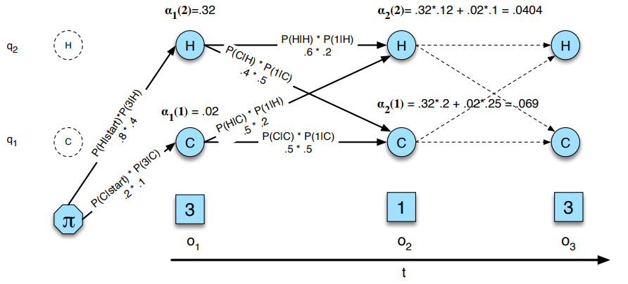
It is done simply by following the different paths in the graph and summing the probabilities of each path.

The very first step is to compute the forward probabilities at time $t = 1$, which is simply the product of the initial state probability and the emission probability of the first observation: $\alpha_{1}(j) = \pi_{j} \times B_{j, O_{1}}$

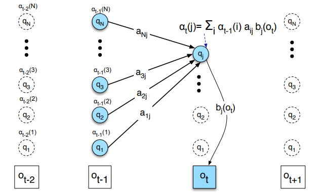
Then, for each time step $t$, we compute the forward probabilities for each state $j$ by summing the probabilities of all paths that lead to state $j$ at time $t$: $\alpha_{t}(j) = \sum_{i=1}^{N} \alpha_{t-1}(i) \times A_{i, j} \times B_{j, O_{t}}$

For a single node, it looks like this:

A simple implementation in Python would look like this where the $\alpha$ matrix is recursively computed:

import numpy as np
def forward_algorithm(pi, O, A, B):
    """
    pi: Initial state proability distribution (N)
    O: Observation sequence (length T)
    A: Transition probability matrix (N x N)
    B: Emission probability matrix (N x T)
    
    Iterate over the observation sequence and compute the forward probabilities
    """
    N = len(A)       # Number of states
    T = len(O)       # Length of observation sequence
    
    # Initial state probability * emission probability of first observation
    forward = np.zeros((N, T))
    forward[:, 0] = pi * B[:, O[0] - 1]  # python is 0 indexed so -1 each val
    
    # Compute the forward probabilities for each state at each time step
    for t in range(1, T):
        for s in range(N):
            forward[s, t] = np.sum(forward[:, t - 1] * A[:, s] * B[s, O[t] - 1])
    total_prob = np.sum(forward[:, -1])  # Final probability is just the sum of the alpha_last(j) for all states j
    return total_prob
# forward_algorithm(pi, O, A, B)
# >> 0.0285

There is a nice python package called hmmlearn that deals with Markov processes, we can verify our results like so :

# pip install hmmlearn
from hmmlearn import hmm
gen_model = hmm.CategoricalHMM(n_components=2)  # 2 hidden states
gen_model.startprob_ = pi  # Initial state probability distribution
gen_model.transmat_ = A  # Transition probability matrix
gen_model.emissionprob_ = B  # Emission probability matrix
O_ = np.array(O) - 1  # python is 0 indexed so -1 each val
O_ = O_.reshape(-1, 1)
log_prob = gen_model.score_samples(O_)  # returns the log probability
total_prob = np.exp(log_prob[0])
print(total_prob)
# >> 0.0285

Decoding

Now that we know how to compute the likelihood of a sequence, we’re interested in finding the most likely sequence of hidden states that generated the observation sequence.
To continue with our example, we want to find the most likely sequence of hidden states that generated the observation sequence $3, 1, 3$ (spoilers : it’s hot cold hot).

What we could do, is to compute the likelihood of all possible sequences of hidden states and choose the one with the highest probability. But that’s not great. Instead, we can use the Viterbi Algorithm, another dynamic programming method.

Viterbi Algorithm

If I understand correctly, the Viterbi algorithm is identical to the forward algorithm but instead of summing the probabilities of all paths that lead to state $j$ at time $t$, we take the maximum probability of all paths that lead to state $j$ at time $t$. Of course, we also need to keep track of the path that led to the maximum probability, which is done with a backtracking step at the end to find the most likely path, i.e following the most likely path at each time step, i.e : $\text{argmax}(\alpha_{t-1}(i) \times A_{i, j} \times B_{j, O_{t}})$

A simple implementation in Python would look like this:

def viterbi_algorithm(pi, O, A, B):
    """
    pi: Initial state proability distribution (N)
    O: Observation sequence (length T)
    A: Transition probability matrix (N x N)
    B: Emission probability matrix (N x T)
    
    Iterate over the observation sequence and compute the forward probabilities
    """
    N = len(A)       # Number of states
    T = len(O)       # Length of observation sequence
    
    viterbi = np.zeros((N, T))
    backtrack = np.zeros((N, T))
    
    viterbi[:, 0] = pi * B[:, O[0] - 1]  # python is 0 indexed so -1 each val
    backtrack[:, 0] = 0
    
    for t in range(1, T):
        for s in range(N):
            delta = viterbi[:, t - 1] * A[:, s] * B[s, O[t] - 1]
            viterbi[s, t] = np.max(delta)
            backtrack[s, t] = np.argmax(delta)
    best_path_prob = np.max(viterbi[:, -1])
    
    # Backtrack to find the most likely path
    best_path = np.zeros(T, dtype=int)
    best_path[-1] = np.argmax(forward[:, -1])
    for t in range(T - 2, -1, -1):
        best_path[t] = backtrack[best_path[t+1], t+1]
    
    return best_path_prob, best_path

# viterbi_algorithm(pi, O, A, B)
# >> 0.012800000000000004, array([1, 0, 1])

We can verify our results with the hmmlearn package (using the same model as above):

log_prob, best_path = gen_model.decode(O_, algorithm="viterbi")  # log prob because of numerical stability n what not
print(np.exp(log_prob), best_path)
# >> 0.012799999999999997 [1 0 1]

Training

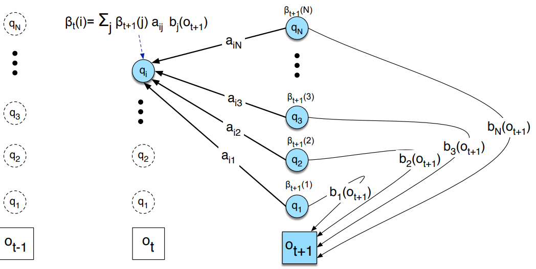
Goal is to learn the matrices $A$ and $B$, we do this with the Baum-Welch Algorithm, an iterative method and special case of Expectation-Maximization. First we need to define the backward probabilities, which are the probability of observing the sequence $O_{t+1}, O_{t+2}, \ldots, O_{T}$ given that we are in state $i$ at time $t$, noted $\beta_{t}(i)$, the computation is identical to the forward probabilities but in reverse.

def backward_algorithm(pi, O, A, B):
    """
    pi: Initial state proability distribution (N)
    O: Observation sequence (length T)
    A: Transition probability matrix (N x N)
    B: Emission probability matrix (N x T)
    
    Iterate over the observation sequence and compute the backward probabilities
    """
    N = len(A)       # Number of states
    T = len(O)       # Length of observation sequence
    
    backward = np.zeros((N, T))
    backward[:, -1] = 1  # Initialization
    
    for t in range(T - 2, -1, -1):
        for s in range(N):
            backward[s, t] = np.sum(backward[:, t + 1] * A[s, :] * B[:, O[t + 1] - 1])
    return backward

Baum-Welch Algorithm

def baum_welch(pi, O, A, B, n_iter=100):
    """
    pi: Initial state proability distribution (N)
    O: Observation sequence (length T)
    A: Transition probability matrix (N x N)
    B: Emission probability matrix (N x T)
    n_iter: Number of iterations
    
    Train the model using the Baum-Welch algorithm
    """
    N = len(A)       # Number of states
    T = len(O)       # Length of observation sequence
    
    for _ in range(n_iter):
        # Compute forward and backward probabilities
        forward = forward_algorithm(pi, O, A, B)
        backward = backward_algorithm(pi, O, A, B)
        
        # Compute the gamma probabilities
        gamma = forward * backward / np.sum(forward * backward, axis=0)
        
        # Compute the xi probabilities
        xi = np.zeros((N, N, T - 1))
        for t in range(T - 1):
            for i in range(N):
                for j in range(N):
                    xi[i, j, t] = forward[i, t] * A[i, j] * B[j, O[t + 1] - 1] * backward[j, t + 1]
            xi[:, :, t] /= np.sum(xi[:, :, t])
        
        # Update the model parameters
        pi = gamma[:, 0]
        for i in range(N):
            for j in range(N):
                A[i, j] = np.sum(xi[i, j, :]) / np.sum(gamma[i, :-1])
        
        for j in range(N):
            for k in range(B.shape[1]):
                B[j, k] = np.sum(gamma[j, O == k]) / np.sum(gamma[j, :])
    
    return pi, A, B

Putting it all together : concrete example on stock prices

Am I rich yet ?

No lol, thanks for reading

Resources

https://web.stanford.edu/~jurafsky/slp3/A.pdf https://github.com/Bratet/Stock-Prediction-Using-Hidden-Markov-Chains/blob/main/src/utils/hmm.py