Trading Crap
Bridgewater (4% returns) vs index funds (18%).
— Sam Parr (@thesamparr) October 7, 2024
I'm not saying you can't beat the market.
But Bridgewater is a hedge fund with 2,000 employees. Some of the smartest, highest paid people on earth who spend 20 hours a day + billions on tools/research.
And they, and many just… pic.twitter.com/YKLzZaikbb
I’ve seen this tweet recently comparing returns of some hedge fund and a passive index fund, besides missing the point of what hedge funds are for (hedging downside risk while trying to keep up with or beat the market), I feel it’s a good excuse to learn some basic risk management and indicators, arguably more important than your PnL.
Data stuff
Just pull some trading data from your favorite exchange, the formating should be relatively similar. I’m only using 1 month worth of trading for simplicity.
import pandas as pd
from datetime import datetime, timedelta

# Load the data
trade_history = pd.read_csv("trade_history.csv")
# Make sure the time column is a datetime object
trade_history['time'] = pd.to_datetime(trade_history['time'], format='%m/%d/%Y - %H:%M:%S')
# Only keep the last month of trading
trade_history = trade_history[(trade_history['time'] >= (datetime.now() - timedelta(days=30)))]
trade_history.head() should look something like this:
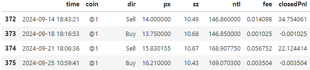
With time being the timestamp of the trade, coin the symbol you’re trading, dir the direction of the trade (buy or sell), px the price, sz the size of the trade (number of coins), ntl the notional value of the trade (size * price), fee the fee paid for the trade which is accounted for in the closedPnl, your profit or loss for the given trade.
Max Drawdown
The maximum drawdown is the maximum loss from a peak to a trough of a portfolio, which is a decent measure of volatility and risk. If you have an insane drawdown, that means that you’re probably taking too much risk and are willing to accept a lot of volatility 👽
# Keep track of the cumulative pnl and the maximum value it has reached at any point of time
trade_history['cumulative_pnl'] = trade_history['closedPnl'].cumsum()
trade_history['rolling_max'] = trade_history['cumulative_pnl'].cummax()

# Drawdown for each trade is how far the cumulative pnl is from the rolling max (peak)
trade_history['drawdown'] = trade_history['rolling_max'] - trade_history['cumulative_pnl']

# The maximum drawdown is simply the max over each trade's drawdown (peak to valley)
max_drawdown = trade_history['drawdown'].max()
print(f"Max drawdown : {max_drawdown:.1f} USD")
# >>> Max drawdown : 41.1 USD
In this toy example, the max drawdown is 41.1 USD, which means that at some point in the last month, the portfolio was down 40 bucks from its peak value.
Sharpe Ratio
The Sharpe ratio is a measure of risk-adjusted return, which is the average return earned in excess of the risk-free rate per unit of volatility or total risk. It’s a good measure to compare different strategies or portfolios, the higher the Sharpe ratio, the better the risk-adjusted return.
^What this chatgpt verbiage is saying is that the sharpe ratio compares your return to something risk-free, divided by the volatility. To maximize the sharpe ratio, you want to maximize your return against the default risk-free and minimize your volatility (Nb : usually, it makes more sense to use this ratio to compare 2 strats rather than a standalone number).
We can start by computing few useful stats :
# Group by timestamp and sum to get total PNL / size per timestamp (day)
daily_pnl = trade_history.groupby(trade_history['time'].dt.date)['closedPnl'].sum()  # PNL in USD
daily_size = trade_history.groupby(trade_history['time'].dt.date)['ntl'].sum()  # Size in USD

# Daily returns as a percentage of the size trade
daily_returns = daily_pnl / daily_size

# Min - max - average - standard deviation of daily returns
avg_daily_return = daily_returns.mean()
min_daily_return = daily_returns.min()
max_daily_return = daily_returns.max()
daily_std = daily_returns.std()

print(f"Average daily returns : {avg_daily_return:.2%} (std : {daily_std:.2%} -- min : {min_daily_return:.2%} -- max : {max_daily_return:.2%})")
# >>> Average daily returns : 3.40% (std : 7.04% -- min : -0.01% -- max : 23.66%)
Here we can see that we only got wins (min being just a trade fee) (yayy), with an average daily return of 3.4% and a standard deviation of 7.04%, which is a bit high but not too bad.
Now we need to find the risk-free rate, which is usually the return on a US treasury bond, but for simplicity I’ll use $5\%$ annual as a default value (high yield savings account). Since we’re working with daily returns, we need to convert this to a daily rate, which is given by the formula :
# Assuming 5% annual risk free rate
annual_rf_rate = 0.05
daily_rf_rate = (1 + annual_rf_rate) ** (1/365) - 1
The Sharpe ratio is then given by the expected return of the portfolio minus the risk-free rate returns divided by the standard deviation of the portfolio :
\[\text{Sharpe ratio} = \frac{\mathbb{E}(R_p - R_f)}{\sigma_p}\]# How far we stray from the risk-free rate for each trade (daily in our case)
daily_excess_returns = daily_returns - daily_rf_rate
# Expectation(R - Rf)
mean_daily_excess_return = daily_excess_returns.mean()
# Sharpe ratio (daily)
daily_sharpe = mean_daily_excess_return / daily_std
# Sharpe ratio (annualized)
annual_sharpe = daily_sharpe * (365 ** 0.5)
print(f"Daily sharpe : {daily_sharpe:.2f} -- Annual : {annualised_sharpe:.2f}")
# >>> Daily sharpe : 0.48 -- Annual : 9.18
Nb : To annualize the sharpe ratio, you need to multiply the daily sharpe ratio by the square root of the number of trading days in a year (365 in crypto, 252 in tradfi).
Here the annualized Sharpe ratio is 9.18, quite optimistic because of the low sample (few trades over 1 month) but this would mean that for each unit of risk we took, we got 9.18 “units” of return, which would be excellent (if we could sustain it, spoilers : it’s hard).